| Difficult | Execution Time | Data Analysis | Radioactive Sources |
|---|---|---|---|
| Yes | No |
Hardware setup
This experiment guide is referred to the SP5630EN/ENP – Environmental Kit. If you don’t have this kit, choose your own from the following list to visualize the related experiment guide: SG6112A, SG6112B, SG6112E – Educational Kit
Equipment: SP5630EN/ENP – Environmental Kit
| Model | i-Spector- S2570B | Additional Tool |
|---|---|---|
| Description | radiation detector systems | Gamma Radioactive Source |
Purpose of the experiment
Study the statistical distribution of the counting rates of a gamma radioactive source. Comparison of the data to the Poisson distribution, turning into a Gaussian as the mean number of counts grows.
Fundamentals
The number of radioactive particles detected over a time Δt is expected to follow a Poisson distribution with mean value μ. It means that for a given radioactive source, the probability that n decays will occur over a given time period Δt is given by:
![]()
Where μ is proportional to the sample size and to the time Δt and inversely proportional to the half-life T1/2 of the unstable nucleus. As long as μ grows, the probability P μ(n) is well approximated by a Gaussian distribution:
![]()
Where σ = √μ is the standard deviation.
Carrying out the experiment

Experimental setup block diagram.
- Put the i-Spector digital into the base and place the radioactive sample, like, for example, the LYSO crystal which is provided as calibration source.
- Power on the i-Spector and connect the Ethernet cable. Wait until the temperature is stable from the web interface (it can take half an hour from power on).
- Check the waveform, modify the threshold and gate width, if needed, then start the measurement of the energy spectrum.
- Take for example 2 minutes of acquisition with the LYSO crystal sample by setting the corresponding acquisition time.
- Select the ROI peak at 303 keV, then check the value reported in the ROI area.
- Repeat the experiment many times and report the ROI area.
Results
Changing the counting window and/or the activity of the source or the ROI, the number of counts changes, with a probability density function moving from a Poissonian to a Gaussian shape. The user may play with the data, fitting them and comparing the expectations to the measurement. The results below have been acquired with 100 consecutive measurements, where the first 30 were used for the Poissonian distribution.![]()
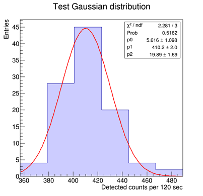
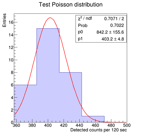
Poissonian distribution [Fit: y = p0* (p1x/x!)*e-p1] on the left, Gaussian distribution on the right.